General introduction

MrIML is a R package allows users to generate and interpret multi-response models (i.e., joint species distribution models) leveraging advances in data science and machine learning. MrIML couples the tidymodel infrastructure developed by Max Kuhn and colleagues with model agnostic interpretable machine learning tools to gain insights into multiple response data such as. As such MrIML is flexible and easily extendable allowing users to construct everything from simple linear models to tree-based methods for each response using the same syntax and same way to compare predictive performance.In this vignette we will guide you through how to apply the MrIML framework to identify and benchmark biosecurity practices in veterinary disease. This working example is built upon a classification framework. More information about this can be found in the “Classification working example”.

Lets load that data

This is a synthesized dataset to simulate PRRSV infection, biosecurity practices and farm demographics on swine farms across the united states. Please note that the data included in this package is simulated, and is not a reflection of any real farm, company or state.

#other packages needed
library(mrIML);library(parsnip);
#> Warning: package 'parsnip' was built under R version 3.6.3
library(tidymodels); library(workflows);
#> Warning: package 'tidymodels' was built under R version 3.6.3
#> Warning: package 'broom' was built under R version 3.6.3
#> Warning: package 'dials' was built under R version 3.6.3
#> Warning: package 'scales' was built under R version 3.6.3
#> Warning: package 'dplyr' was built under R version 3.6.3
#> Warning: package 'ggplot2' was built under R version 3.6.3
#> Warning: package 'infer' was built under R version 3.6.3
#> Warning: package 'modeldata' was built under R version 3.6.3
#> Warning: package 'purrr' was built under R version 3.6.3
#> Warning: package 'recipes' was built under R version 3.6.3
#> Warning: package 'rsample' was built under R version 3.6.3
#> Warning: package 'tibble' was built under R version 3.6.3
#> Warning: package 'tidyr' was built under R version 3.6.3
#> Warning: package 'tune' was built under R version 3.6.3
#> Warning: package 'workflows' was built under R version 3.6.3
#> Warning: package 'workflowsets' was built under R version 3.6.3
#> Warning: package 'yardstick' was built under R version 3.6.3
library(tidyverse); library(flashlight);
#> Warning: package 'tidyverse' was built under R version 3.6.3
#> Warning: package 'readr' was built under R version 3.6.3
#> Warning: package 'stringr' was built under R version 3.6.1
#> Warning: package 'forcats' was built under R version 3.6.3
#> Warning: package 'flashlight' was built under R version 3.6.3
library(devtools); library(DALEX); 
#> Warning: package 'devtools' was built under R version 3.6.3
#> Warning: package 'usethis' was built under R version 3.6.3
#> Warning: package 'DALEX' was built under R version 3.6.3
library(plyr);library(vip);
#> Warning: package 'plyr' was built under R version 3.6.3
#> Warning: package 'vip' was built under R version 3.6.3
library(ggsci); library(ggrepel);
#> Warning: package 'ggsci' was built under R version 3.6.1
#> Warning: package 'ggrepel' was built under R version 3.6.3
library(breakDown); library(future.apply);
#> Warning: package 'breakDown' was built under R version 3.6.3
#> Warning: package 'future.apply' was built under R version 3.6.3
#> Warning: package 'future' was built under R version 3.6.3
library(janitor)
#> Warning: package 'janitor' was built under R version 3.6.3

set.seed(130) #set the seed to ensure consistency
data <- as.data.frame(mrIML::biosecurity_vignette_data)

Defining your model engine

This is a random forest model, as used in the classification example. However there are more models available within MrIML and can be found here.

#split predictor variables and outcome
Y <- as.data.frame(data %>% select(1))
X <- data %>% select(-c(1, 44, 45)) #remove class, group and ID
model1 <- #model used to generate yhat
  #specify that the model is a random forest
  rand_forest(trees = 100, mtry = tune(), min_n = tune(), mode = "classification") %>% 
  #select the engine/package that underlies the model
  set_engine("ranger", importance = c("impurity","impurity_corrected")) %>%
  #must be set to classification for classification problems
  set_mode("classification")

###Parallel processing

MrIML provides uses the flexible future apply functionality to set up multi-core processing. In the example below, we set up a cluster using 4 cores. If you don’t set up a cluster, the default settings will be used and the analysis will run sequentially.

# detectCores() #check how many cores you have available. We suggest keeping one core free for internet browsing etc.

cl <- parallel::makeCluster(4)

plan(cluster, workers=cl)

Running the analyis

Now we can train and test our model.

yhats <- mrIMLpredicts(X=X, #features/predictors 
                       Y=Y, #response data
                       Model=model1, #specify your model
                       balance_data='no', #chose how to balance your data 
                       mode='classification', #chose your mode (classification versus regression)
                       seed = 120) #set seed

We can then assess our model performance using a number of performance metrics including area under the curve (AUC), sensitivity, specificity and Matthews correlation coefficient (MCC).

ModelPerf <- mrIMLperformance(yhats=yhats, Model=model1, Y=Y, mode='classification')
ModelPerf[[1]] #predictive performance for individual responses 
#>   response  model_name           roc_AUC               mcc       sensitivity
#> 1    Class rand_forest 0.695652173913043 0.436392914653784 0.740740740740741
#>         specificity prevalence
#> 1 0.695652173913043        0.5
ModelPerf[[2]]#overall predictive performance. r2 for regression and MCC for classification
#> [1] 0.6956522

Benchmarking: global importance

Here we can look at the variable importance. This is the dependence between our outcome and biosecurity variables.

#calculate variable importance
VI <- mrVip(yhats=yhats, X=X)
#plot cumulative variable importance 
plot_vi_biosecurity(VI=VI, Y=Y, X=X,
        modelPerf=ModelPerf,
        cutoff= 0.6,
        plot.pca='no') #Follow instructions in console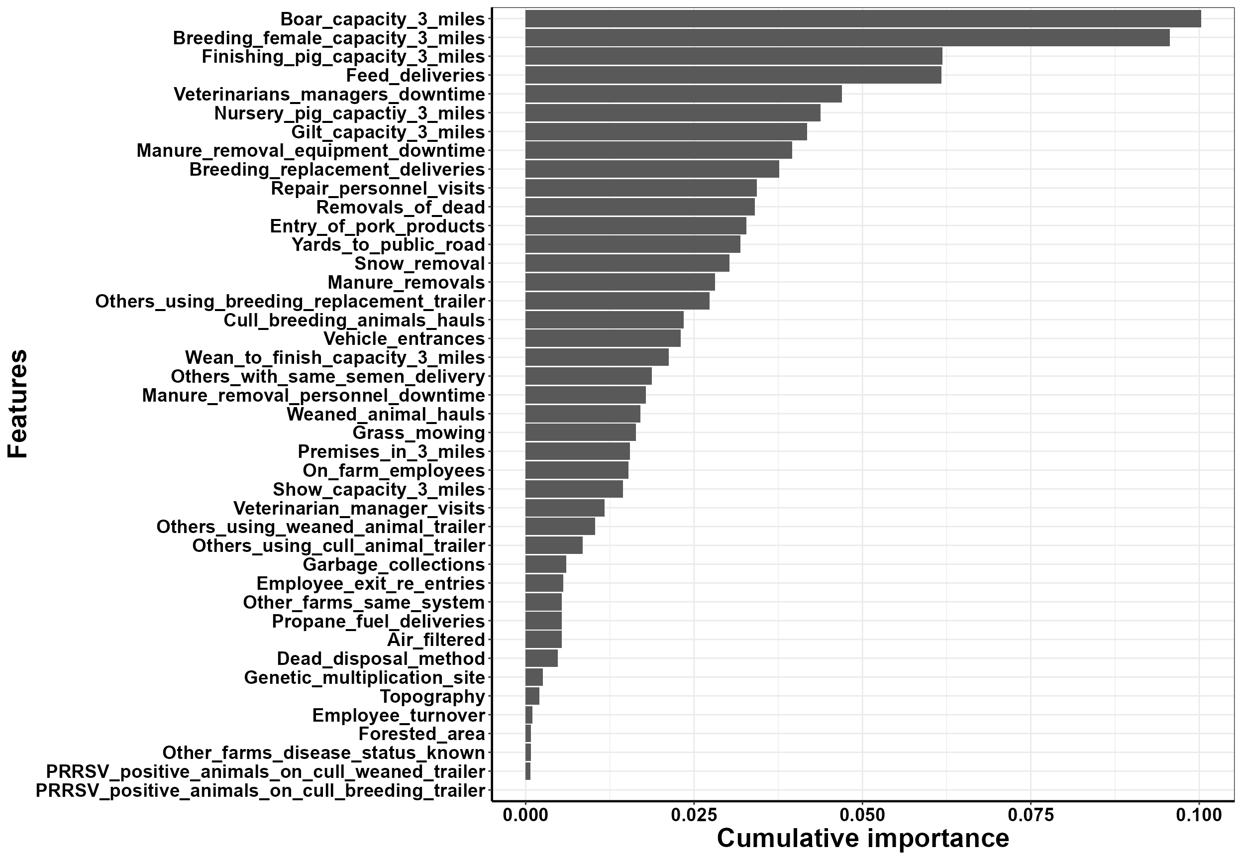

#> Press [enter] to plot individual variable importance summaries
#> [1] ""

We can explore further and assess the partial dependence of each variable. Here we isolate the dependence of one variable and visualize how this dependence changes over different observed values.

#create a flashlight object
fl <- mrFlashlight(yhats=yhats, X=X, Y=Y, 
                   response="single", 
                   index=1,
                   mode='classification') 
#plot partial dependence profiles
plot(light_profile(fl, v = "Premises_in_3_miles"))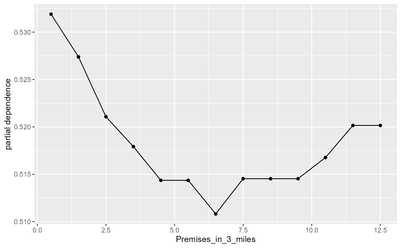

Benchmarking: predicted risk

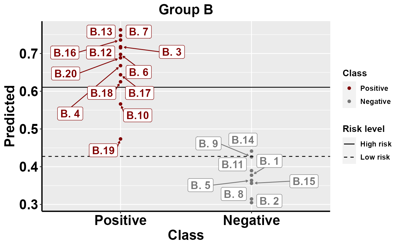
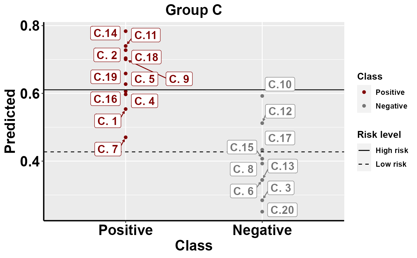
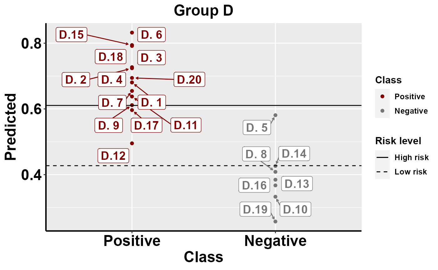
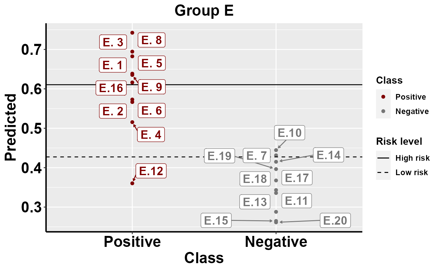
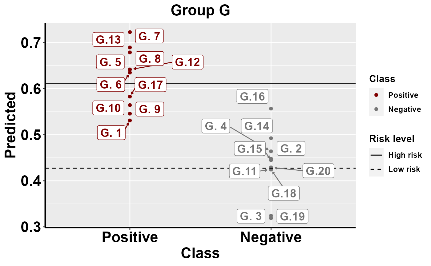
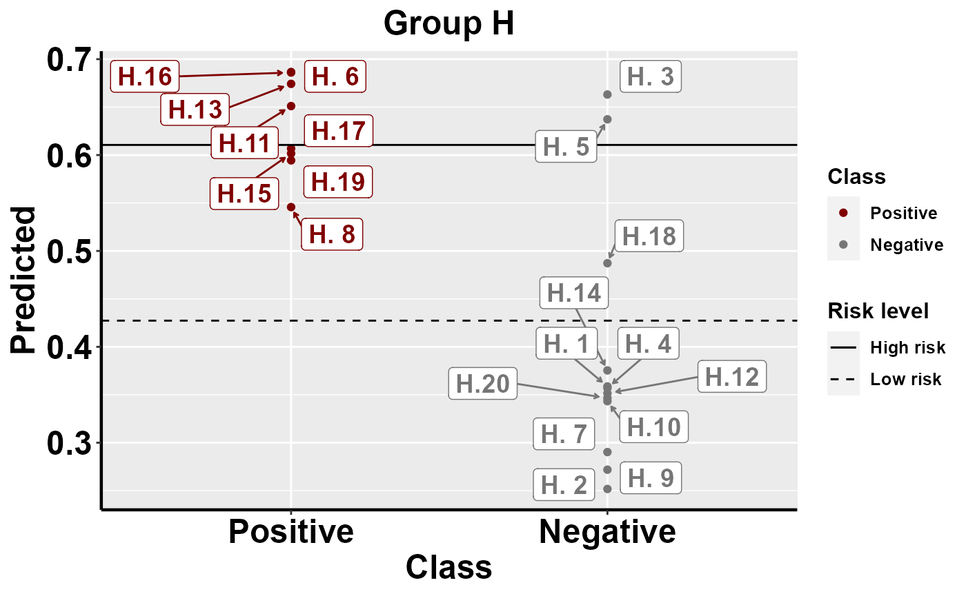
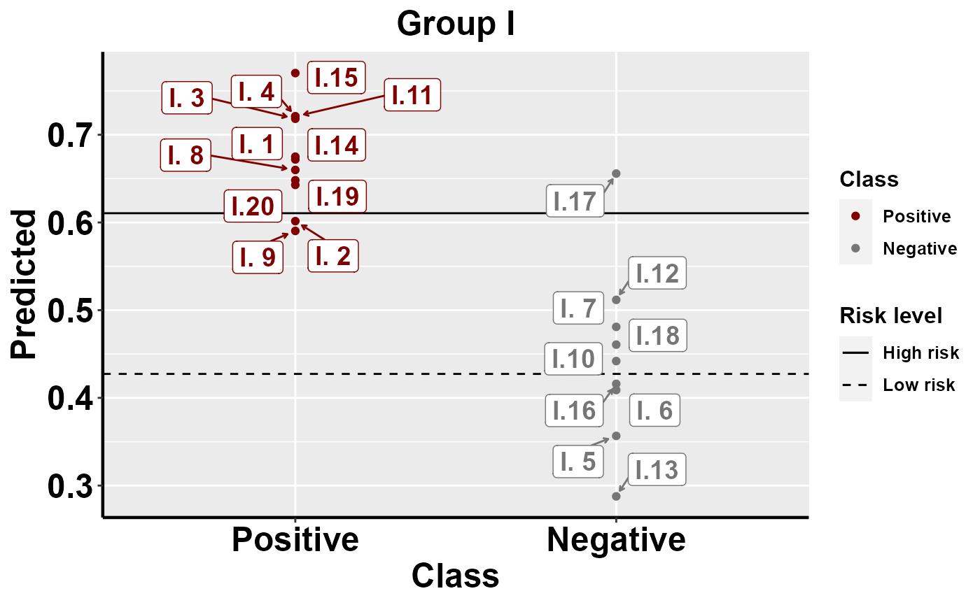
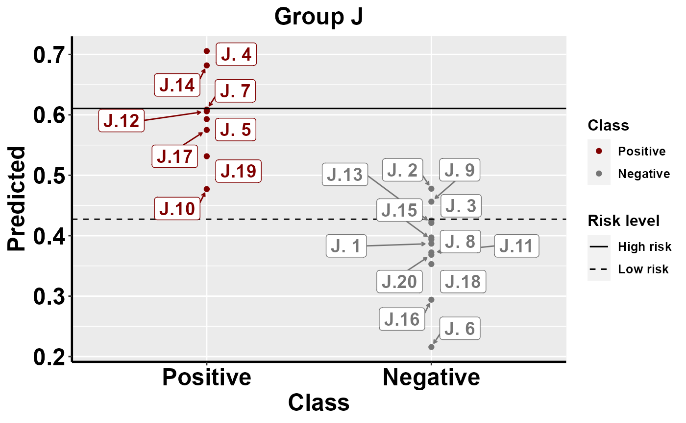
The following function allows you to visualize and compare predicted risk among and within groups

#apply the trained model to the entire data set to provide risk of predicted outbreak
fit_bio <- pull_workflow_fit(yhats[[1]]$mod1_k)
preds_pos <- predict(fit_bio, data, "prob")
data$Predicted <- preds_pos$.pred_1
#process data ready for the function
data$Class <- as.factor(data$Class)
data<-data%>%
  mutate(Class = revalue(Class,
                         c("1" = "Positive", "0" = "Negative"))) 
data$Class <- relevel(data$Class, "Positive")
data1 <- data
#plot among group comparison of predicted risk
mrBenchmark(data = "data1", Y = "Class", pred = "Predicted", group = "Group", type = "external")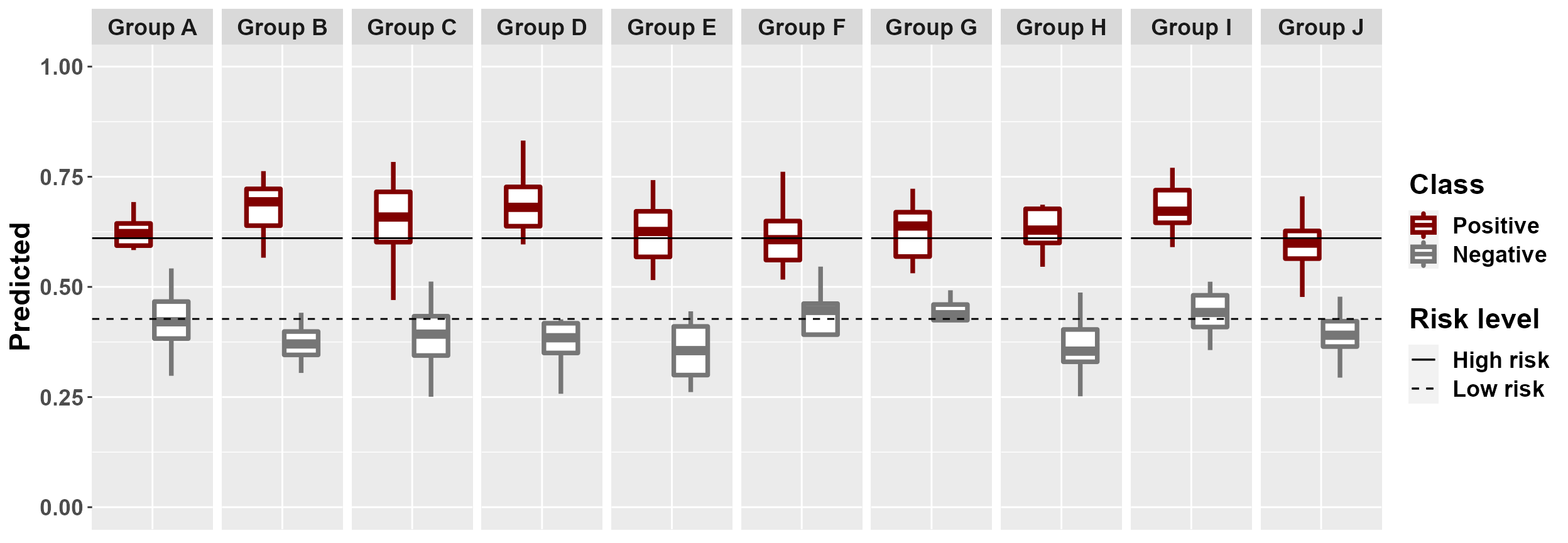

#plot within group comparison of predicted risk
mrBenchmark(data = "data1", Y = "Class", pred = "Predicted", group = "Group", label_by = "ID", type = "internal")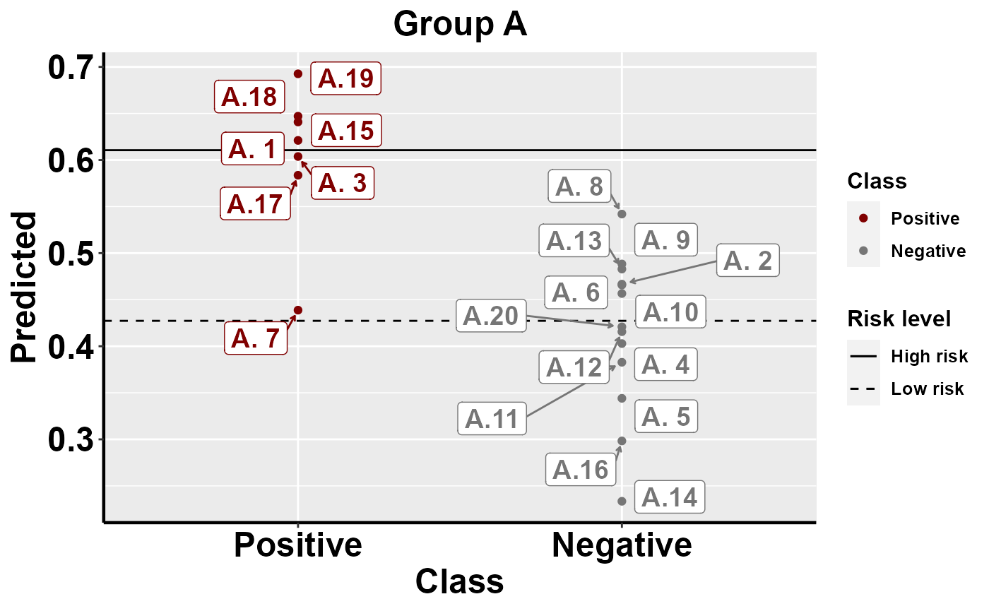

Benchmarking: local importance

To investigate and interpret the contribution of variables at an individual level, we must use a local explanation method. Here we implement a local breakDown explainer. mrLocalExplainer produces both aggregated and individual results of variable contribution. Variables with a phi > 0 contribute to an increase in predicted PRRSV outbreak risk, while variables with a phi < 0 contribute to a decrease in predicted outbreak risk.

#Use this function to implement the local explainer 
data<-data%>%
  mutate(Class = revalue(Class,
                         c("1" = "Positive", "0" = "Negative"))) 
data$Class <- relevel(data$Class, "Positive")
X1 <- X
mrLocalExplainer(X = X1, Model = yhats, Y = data$Class)
#> Preparation of a new explainer is initiated
#>   -> model label       :  ranger  ( [33m default [39m )
#>   -> data              :  200  rows  42  cols 
#>   -> target variable   :  not specified! ( [31m WARNING [39m )
#>   -> predict function  :  yhat.ranger  will be used ( [33m default [39m )
#>   -> predicted values  :  No value for predict function target column. ( [33m default [39m )
#>   -> model_info        :  package ranger , ver. 0.12.1 , task classification ( [33m default [39m ) 
#>   -> model_info        :  Model info detected classification task but 'y' is a NULL .  ( [31m WARNING [39m )
#>   -> model_info        :  By deafult classification tasks supports only numercical 'y' parameter. 
#>   -> model_info        :  Consider changing to numerical vector with 0 and 1 values.
#>   -> model_info        :  Otherwise I will not be able to calculate residuals or loss function.
#>   -> predicted values  :  numerical, min =  0.2157556 , mean =  0.5195907 , max =  0.8321314  
#>   -> residual function :  difference between y and yhat ( [33m default [39m )
#>  [32m A new explainer has been created! 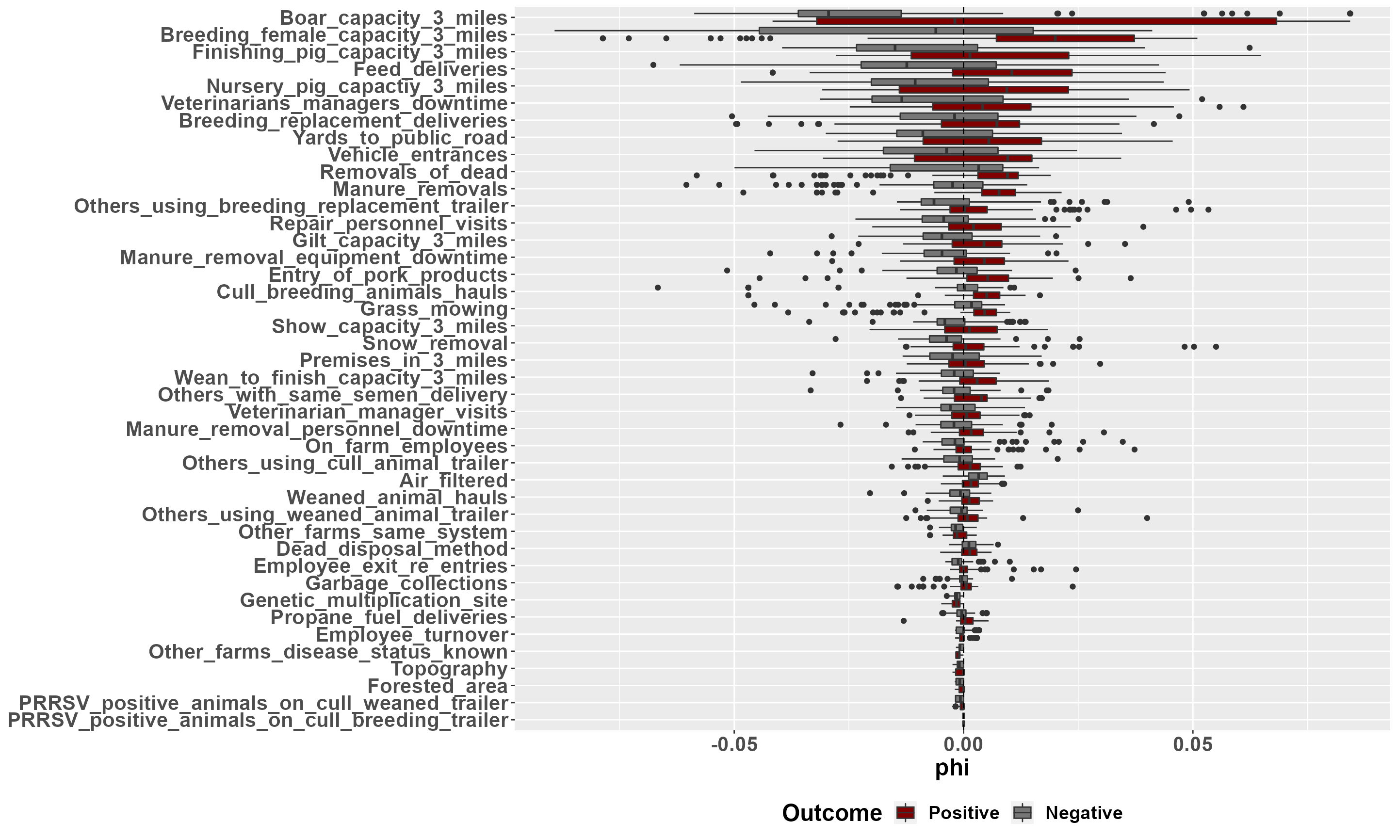[39m

Individual plots are produced in the list object LE_indiv_plots. Each plot corresponds to a single farm. An example of a positive farm and a negative farm are shown here.

LE_indiv_plots[1]
#> [[1]]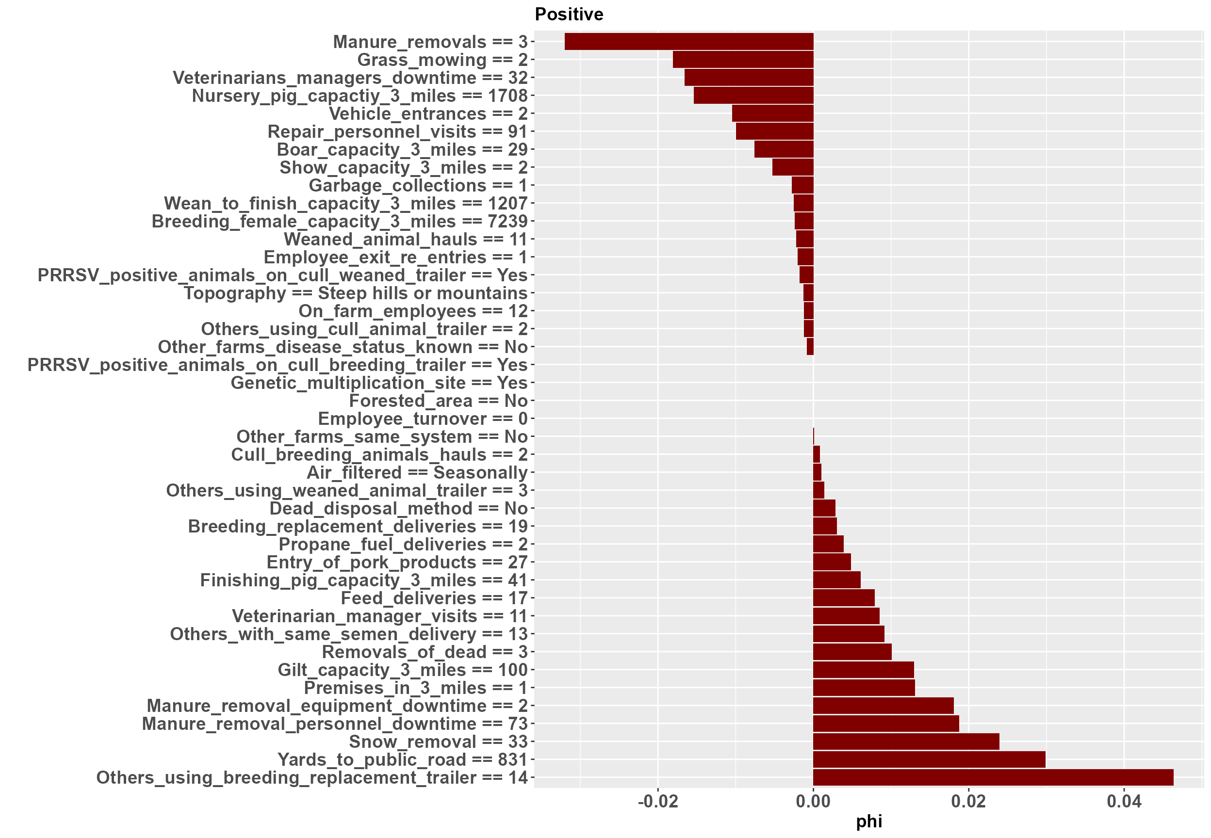

LE_indiv_plots[2]
#> [[1]]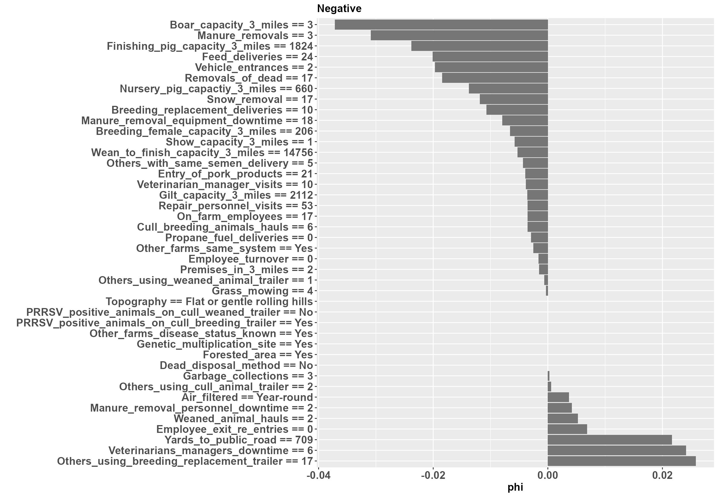

At the positive farm we can see that yards from the public road and garbage collection are contributing to an increased outbreak risk, while manure removals and repair visits are contributing to a decreased outbreak risk. Likewise, at the negative farm yards to the public road and and the downtime required for manure removal personnel are contributing to an increased outbreak risk, while feed deliveries and manure removals are contributing to a decreased outbreak risk.

This session of the MrIML has been funded by Critical Agricultural Research and Extension 2019-68008-29910 from the USDA National Institute of Food and Agriculture.

Biosecurity working example

Abagael Sykes, Gustavo Machado