MrIML is a R package allows users to generate and interpret multi-response models (i.e., joint species distribution models) leveraging advances in data science and machine learning. MrIML couples the tidymodel infrastructure developed by Max Kuhn and colleagues with model agnostic interpretable machine learning tools to gain insights into multiple response data such as. As such mrIML is flexible and easily extendable allowing users to construct everything from simple linear models to tree-based methods for each response using the same syntax and same way to compare predictive performance. In this vignette we will guide you through how to apply this package to landscape genetics problems but keep in mind any multiple-response data can be interrogated using this package (e.g., species or OTU presence/absence data).
Let’s start by loading the required packages and data. The data we are going to use is from Fountain-Jones etal (2017) and consists of single nucleotide polymorphism (SNP) data from a virus (feline immunodeficiency virus, FIV) infecting bobcats in Southern California.
Features (a.k.a predictor variables) with missing data can be removed or interpolated depending on the nature of the missing data. Here we remove them.
When constructing these type of models, SNPs that are common (occur say in >80% of samples) or rare (< 10% of samples) are difficult to model. This cn be a problem for potentially adaptice loci which tend to be rarer We provide down-sampling or up-sampling strategies for dealing with unbalanced data (see below) but filtering out common and rare loci is another option. The more response variables (SNPs) you include the longer the computational time, so for this example we will trim SNPs occurring in < 40% and > 70% of individuals. This leaves 29 SNPs remaining. In practice, these filtering steps are stringent so < 20 and > 80 maybe more appropriate.
#Optional: Filter rare/common SNPs or species. Retaining minor allelle frequncies >0.1 and removing common allelles (occur>0.9)
fData <- filterRareCommon (Responsedata,
                           lower=0.4,
                           higher=0.7)
Y <- fData #for simplicity when comparing

#another option at this stage is to filter response that are strongly correlated with each other.
#df2 <- cor(X) #find correlations
#hc <-  findCorrelation(df2, cutoff=0.5) # put any value as a "cutoff".
#hc <-  sort(hc)
#X <-  X[,-c(hc)] #
If your feature data consists of landscape resistance data generated from Circuitscape or similar, we provide functionality that can extract each surface from a folder and generate resistance components that can be used in these models (using principal coordinate analysis). This data can be easily merged if needs be with other non-matrix data (e.g., age/sex). There was no resistance surfaces here, but this is what the code looks like:
R <- resist_components(filename = 'location of pairwise matrices', p_val=0.01 ) # p values are used here to filter resistance components that aren't correlated with th original pairwise matrix.
X<- cbind(R,X)
Now all the data is loaded and ready to go we can formulate the model using tidymodel syntax. In this case we have binary data (SNP presence/absence at each loci) but the data could also be counts or continuous (the set_model argument would be “regression” instead of “classification”). The user can specify any model from the tidymodel universe as ‘model 1’ (see https://www.tidymodels.org/find/ for details). However, we have done most of our testing on random forests (rf), xgr boost and glms (generalized linear models). Here we will specify a random forest classification model as the model applied to each response.
model_rf <- rand_forest(trees = 100,
              mode = "classification",
              mtry = tune(),
              min_n = tune()) %>% #100 trees are set for brevity. Aim to start with 1000
          set_engine("randomForest")

#we are tuning mtry and min_n
#set up parallel processing. If you don't add the code below it will still work but just on one core.

## detectCores() #check how many cores you have available. We suggest keeping one core free for internet browsing etc.

cl <- parallel::makeCluster(4)
plan(cluster, workers=cl)
Now we can run the model. Hyper parameter tuning (for algorithms that have hyper parameters) is done automatically by testing how model performance changes across a random grid of 10 parameters and the best performing combination is kept. The only choice to make is to either down/up sample data or leave it as is. As our viral data set is small, we will not do any up or down-sampling (option ‘no’). We could also implement parallel processing for larger data sets.
yhats_rf <- mrIMLpredicts(X=X,
                          Y=Y,
                          Model=model_rf,
                          balance_data='no',
                          mode='classification',
                          k=5,
                          tune_grid_size=5,
                          seed=123,
                          racing=F) ## in MrTidymodels. Balanced data= up upsamples and down downsampled to create a balanced set

# save the model
#save(yhats, file='rf_model')
It takes a couple of minutes to run on a laptop and there are warnings that you can ignore (this data set is small). The above code constructs tuned random forest models for the features (Y) you have selected for each response (29 viral SNP in this case). We can then check the performance of each model separately and overall. The performance metrics we provide for classification models are area under curve (roc_AUC), Mathew’s correlation coefficient (MCC - a good metric when data is imbalanced i.e., unequal numbers of 0/1s in each response), specificity (proportion correctly classified not having the mutation at that loci) and sensitivity (proportion correctly classified having the mutation at that loci). We also provide ‘prevalence’ that tells you how common that SNP was in the population sampled.
ModelPerf_rf <- mrIMLperformance(yhats_rf,
                                 Model=model_rf,
                                 Y=Y,
                                 mode='classification')

ModelPerf_rf[[1]] #predictive performance for individual responses
#>    response  model_name            roc_AUC                mcc       sensitivity
#> 1   env_131 rand_forest  0.642857142857143  0.327326835353989 0.285714285714286
#> 2   env_163 rand_forest  0.238095238095238 -0.327326835353989                 0
#> 3   env_164 rand_forest  0.895833333333333  0.534522483824849               0.5
#> 4   env_167 rand_forest  0.833333333333333               <NA>                 1
#> 5   env_169 rand_forest  0.642857142857143  0.327326835353989 0.285714285714286
#> 6   env_212 rand_forest  0.444444444444444  0.272165526975909                 1
#> 7    env_23 rand_forest               0.48 -0.333333333333333                 0
#> 8    env_24 rand_forest               0.28               <NA>                 1
#> 9    env_41 rand_forest  0.208333333333333 -0.408248290463863 0.333333333333333
#> 10   env_47 rand_forest               0.86  0.816496580927726                 1
#> 11   env_59 rand_forest  0.642857142857143  0.327326835353989 0.285714285714286
#> 12    env_8 rand_forest            0.78125               <NA>                 0
#> 13   env_84 rand_forest  0.642857142857143  0.327326835353989 0.285714285714286
#> 14   env_85 rand_forest  0.642857142857143  0.327326835353989 0.285714285714286
#> 15   env_86 rand_forest             0.4375               <NA>                 1
#> 16  pol_105 rand_forest  0.854166666666667  0.408248290463863 0.333333333333333
#> 17  pol_108 rand_forest  0.761904761904762  0.327326835353989 0.285714285714286
#> 18  pol_111 rand_forest  0.895833333333333  0.534522483824849               0.5
#> 19  pol_117 rand_forest               0.78  0.654653670707977                 1
#> 20  pol_132 rand_forest               0.86  0.816496580927726                 1
#> 21  pol_159 rand_forest               0.28  0.333333333333333                 1
#> 22  pol_258 rand_forest 0.0833333333333333 -0.356348322549899               0.5
#> 23   pol_30 rand_forest               0.86  0.816496580927726                 1
#> 24  pol_340 rand_forest 0.0952380952380952 -0.218217890235992 0.142857142857143
#> 25  pol_353 rand_forest             0.4375               <NA>                 1
#> 26  pol_366 rand_forest  0.642857142857143  0.327326835353989 0.285714285714286
#> 27   pol_87 rand_forest               0.86  0.816496580927726                 1
#> 28   pol_88 rand_forest               0.86  0.816496580927726                 1
#> 29   pol_89 rand_forest               0.86  0.816496580927726                 1
#>                  ppv       specificity        prevalence
#> 1                  1                 1 0.421052631578947
#> 2  0.714285714285714                 0 0.631578947368421
#> 3                  1                 1 0.421052631578947
#> 4                  0               0.4 0.421052631578947
#> 5                  1                 1 0.421052631578947
#> 6  0.444444444444444 0.166666666666667 0.684210526315789
#> 7                0.8                 0 0.631578947368421
#> 8                  0               0.5 0.421052631578947
#> 9               0.25               0.4 0.473684210526316
#> 10               0.8 0.833333333333333 0.473684210526316
#> 11                 1                 1 0.421052631578947
#> 12                 1               NaN 0.473684210526316
#> 13                 1                 1 0.421052631578947
#> 14                 1                 1 0.421052631578947
#> 15                 0               0.4 0.421052631578947
#> 16                 1                 1 0.473684210526316
#> 17                 1                 1 0.421052631578947
#> 18                 1                 1 0.421052631578947
#> 19               0.6 0.714285714285714 0.473684210526316
#> 20               0.8 0.833333333333333 0.473684210526316
#> 21               0.2 0.555555555555556 0.473684210526316
#> 22 0.166666666666667 0.285714285714286 0.473684210526316
#> 23               0.8 0.833333333333333 0.473684210526316
#> 24 0.666666666666667               0.5 0.421052631578947
#> 25                 0               0.4 0.421052631578947
#> 26                 1                 1 0.421052631578947
#> 27               0.8 0.833333333333333 0.473684210526316
#> 28               0.8 0.833333333333333 0.473684210526316
#> 29               0.8 0.833333333333333 0.473684210526316
ModelPerf_rf[[2]]#overall predictive performance
#> [1] 0.2856634
You can compare the predictive performance of random forests with any other technique simply by altering the following. Lets try a logistic regression. Note that for logistic regression you may need to scale/transform the data or create dummy variables if you include categorical variables. These steps can easily be added to the pipeline following tidymodel syntax (see the website above)
model_glm <- #model used to generate yhat
  logistic_reg() %>%
  set_engine("glm") %>%
  set_mode("classification")

yhats_glm <- mrIMLpredicts(X=X,
                           Y=Y,
                           Model=model_glm,
                           balance_data='no',
                           mode='classification',
                           k=5,
                           tune_grid_size=1,
                           seed = sample.int(1e8, 1),
                           racing=F )#no need for a tuning grid - no paramters to tune for logistic regression
#>   |                                                                              |                                                                      |   0%  |                                                                              |==                                                                    |   3%  |                                                                              |=====                                                                 |   7%  |                                                                              |=======                                                               |  10%  |                                                                              |==========                                                            |  14%  |                                                                              |============                                                          |  17%  |                                                                              |==============                                                        |  21%  |                                                                              |=================                                                     |  24%  |                                                                              |===================                                                   |  28%  |                                                                              |======================                                                |  31%  |                                                                              |========================                                              |  34%  |                                                                              |===========================                                           |  38%  |                                                                              |=============================                                         |  41%  |                                                                              |===============================                                       |  45%  |                                                                              |==================================                                    |  48%  |                                                                              |====================================                                  |  52%  |                                                                              |=======================================                               |  55%  |                                                                              |=========================================                             |  59%  |                                                                              |===========================================                           |  62%  |                                                                              |==============================================                        |  66%  |                                                                              |================================================                      |  69%  |                                                                              |===================================================                   |  72%  |                                                                              |=====================================================                 |  76%  |                                                                              |========================================================              |  79%  |                                                                              |==========================================================            |  83%  |                                                                              |============================================================          |  86%  |                                                                              |===============================================================       |  90%  |                                                                              |=================================================================     |  93%  |                                                                              |====================================================================  |  97%  |                                                                              |======================================================================| 100%

#save(yhats, file='logreg_model')
ModelPerf_glm <- mrIMLperformance(yhats_glm,
                                  Model=model_glm,
                                  Y=Y, mode='classification') #
ModelPerf_glm[[2]]
#> [1] 0.06059334

plots <- mrPerformancePlot(ModelPerf1=ModelPerf_glm,
                           ModelPerf2=ModelPerf_rf,
                           mod_names=c('linear_reg','rand_forest'), mode='classification' )
plots
#> [[1]]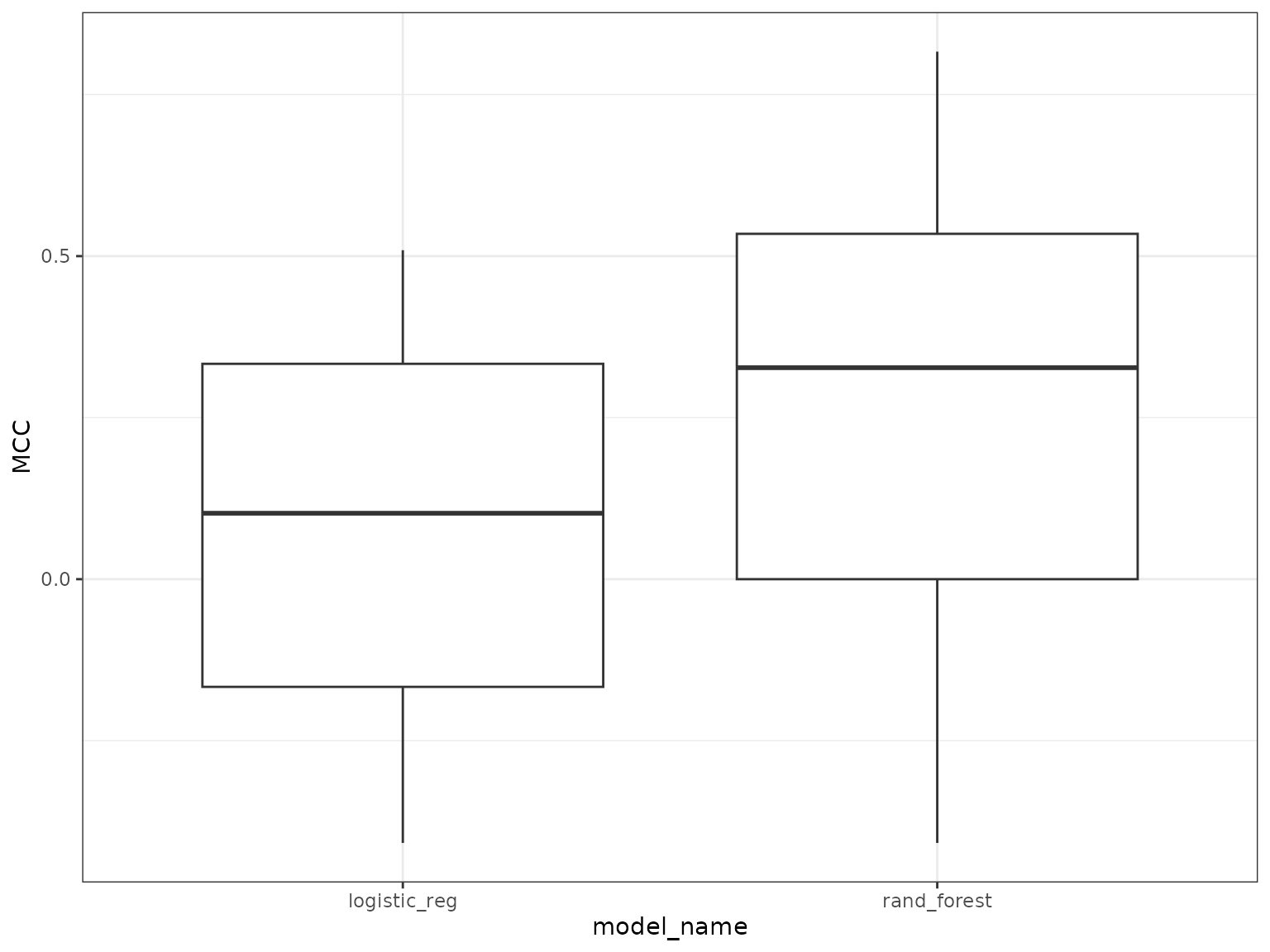
#>
#> [[2]]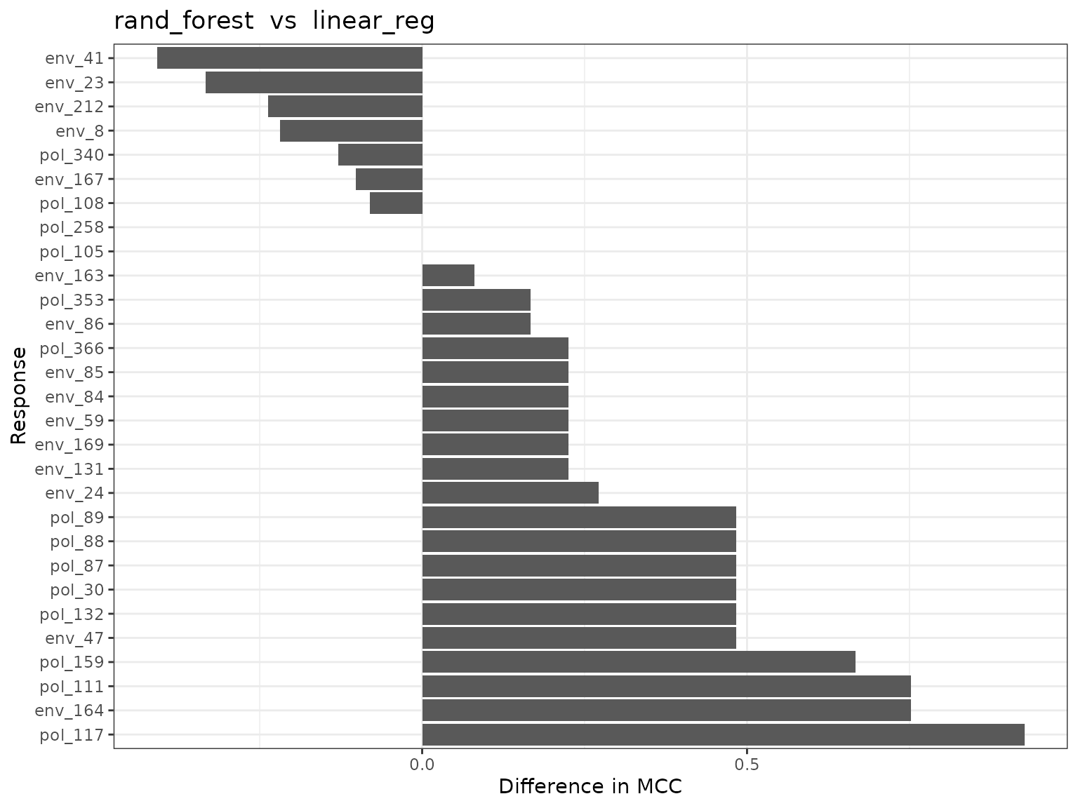
#>
#> [[3]]
#> # A tibble: 29 × 5
#>    response outlier logistic_reg rand_forest diff_mod1_2
#>    <chr>    <lgl>          <dbl>       <dbl>       <dbl>
#>  1 env_131  NA             0.102       0.327      0.225
#>  2 env_163  NA            -0.408      -0.327      0.0809
#>  3 env_164  NA            -0.218       0.535      0.753
#>  4 env_167  NA             0.102       0         -0.102
#>  5 env_169  NA             0.102       0.327      0.225
#>  6 env_212  NA             0.509       0.272     -0.237
#>  7 env_23   NA             0          -0.333     -0.333
#>  8 env_24   NA            -0.272       0          0.272
#>  9 env_41   NA             0          -0.408     -0.408
#> 10 env_47   NA             0.333       0.816      0.483
#> # ℹ 19 more rows
You can see that the random forests model outperforms the logistic regression in this case. Once we are happy with the underlying model we can then dive in to see how this model predicts the SNPs. First we can check out variable importance.The first plot is the global importance (what features shape genetic change overall), the second shows the individual models (with an optional importance MCC threshold ‘cutoff’ value ). The next plot is a PCA plot of the importance scores to highlight SNPs that are potential outliers (predictions are shaped differently by landscape varables).
#bootstrap not working on this small data set.

bs_impVI <- mrvip(
  mrBootstrap_obj = NULL,
  yhats = yhats_rf,
  X = X,
  Y = Y,
  mode = 'classification',
  threshold = 0.8,
  global_top_var = 10,
  local_top_var = 5,
  taxa = 'pol_132',
  ModelPerf = ModelPerf_rf)
#> [1] "here"

bs_impVI[[3]] #importance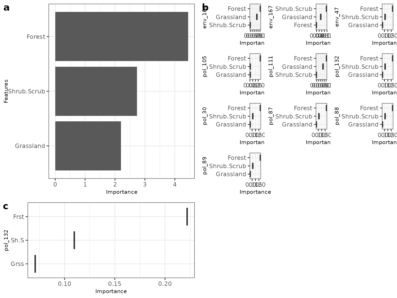
bs_impVI[[4]] #PCA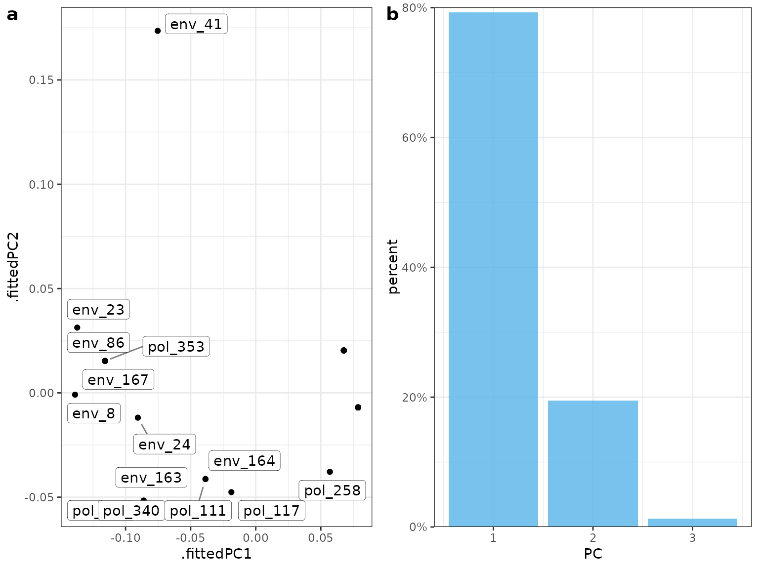 MrIML allows a full suite of model agnostic interpretable machine
learning tools to be applied to individual models or the ‘global’ set.
We utilize the R package flashlight which offers an exciting and ever
growing tool set to interpret these models: https://cran.r-project.org/web/packages/flashlight/vignettes/flashlight.html
MrIML allows a full suite of model agnostic interpretable machine
learning tools to be applied to individual models or the ‘global’ set.
We utilize the R package flashlight which offers an exciting and ever
growing tool set to interpret these models: https://cran.r-project.org/web/packages/flashlight/vignettes/flashlight.html
For example, once we create the flashlight objects, we can plot the predicted values of a feature for each response.
fl <- mrFlashlight(yhats_rf,
X=X,
Y=Y,
response = "single",
index=1,
mode='classification') #index pointing to the SNP of interest (i.e. the first column)
mfl <- mrFlashlight(yhats_rf,
X=X,
Y=Y,
response = "multi",
mode='classification') #the global set
plot(light_scatter(fl, v = "Grassland", type = "predicted"))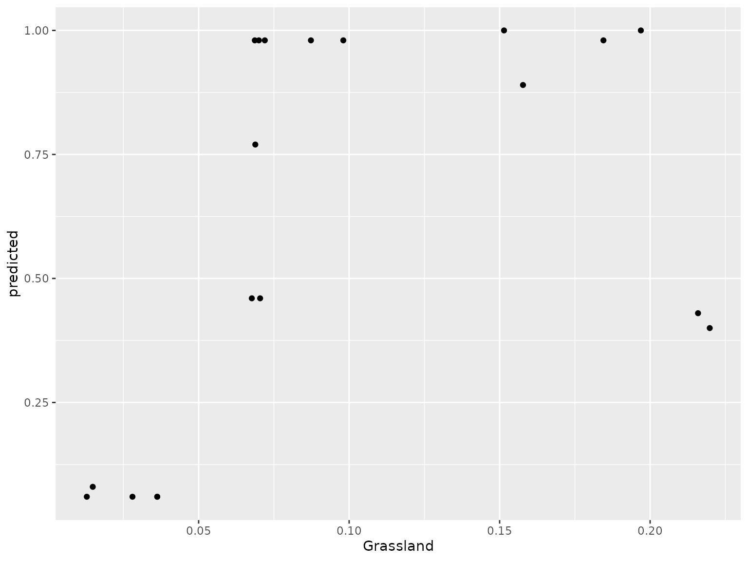 We also wrap some flashlight functionality to visualize the marginal
(i.e. partial dependencies) or conditional (accumulated local effects)
effect of a feature on genetic change. Partial dependencies take longer
to calculate and are more sensitive to correlated features. The first
plot You can see here that they can get different results based on which
plot you use. ALE plots are a better option if your feature set is even
moderately impacted by collinearity ( e.g., ., rho = 0.6). The second
plot is the overall smoothed genetic-turnover function.
We also wrap some flashlight functionality to visualize the marginal
(i.e. partial dependencies) or conditional (accumulated local effects)
effect of a feature on genetic change. Partial dependencies take longer
to calculate and are more sensitive to correlated features. The first
plot You can see here that they can get different results based on which
plot you use. ALE plots are a better option if your feature set is even
moderately impacted by collinearity ( e.g., ., rho = 0.6). The second
plot is the overall smoothed genetic-turnover function.
When running this code yourself, you need to change ‘v’ to the variable of interest within your Y dataset.In this case we are looking at how grassland shapes genetic turnover.
You could easily compare the plots generated above from our random forest model with the logistic regression model we also calculated.
profileData_pd <- light_profile(mfl,
                                v = "Grassland") #partial dependencies
profileData_ale <- light_profile(mfl,
                                 v = "Grassland", type = "ale") #acumulated local effects

mrProfileplot(profileData_pd , sdthresh =0.05) #sdthresh removes responses from the first plot that do not vary with the feature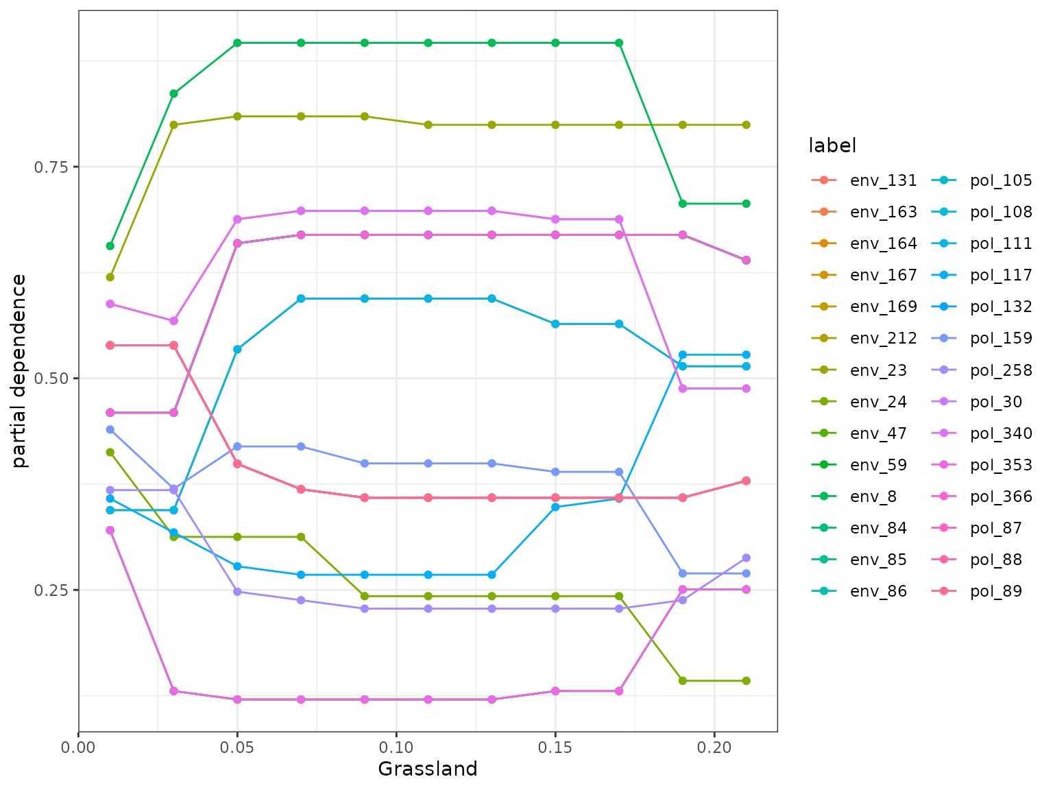
#> Press [enter] to continue to the global summary plot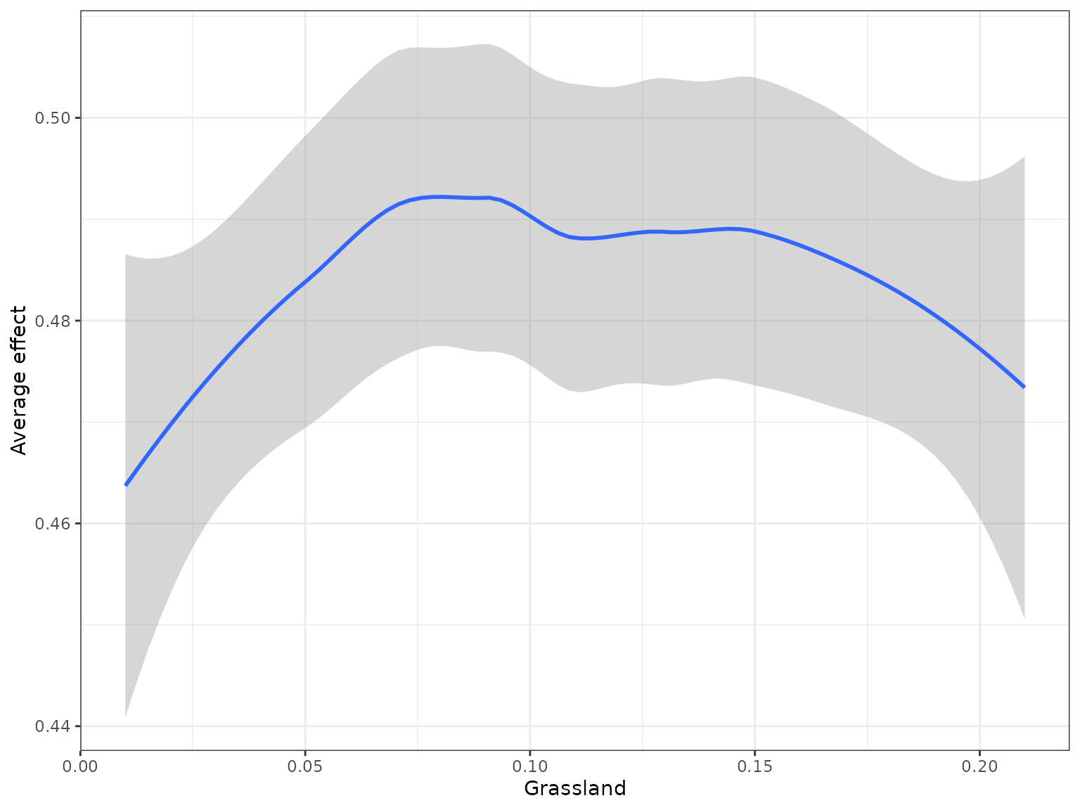
mrProfileplot(profileData_ale , sdthresh =0.05)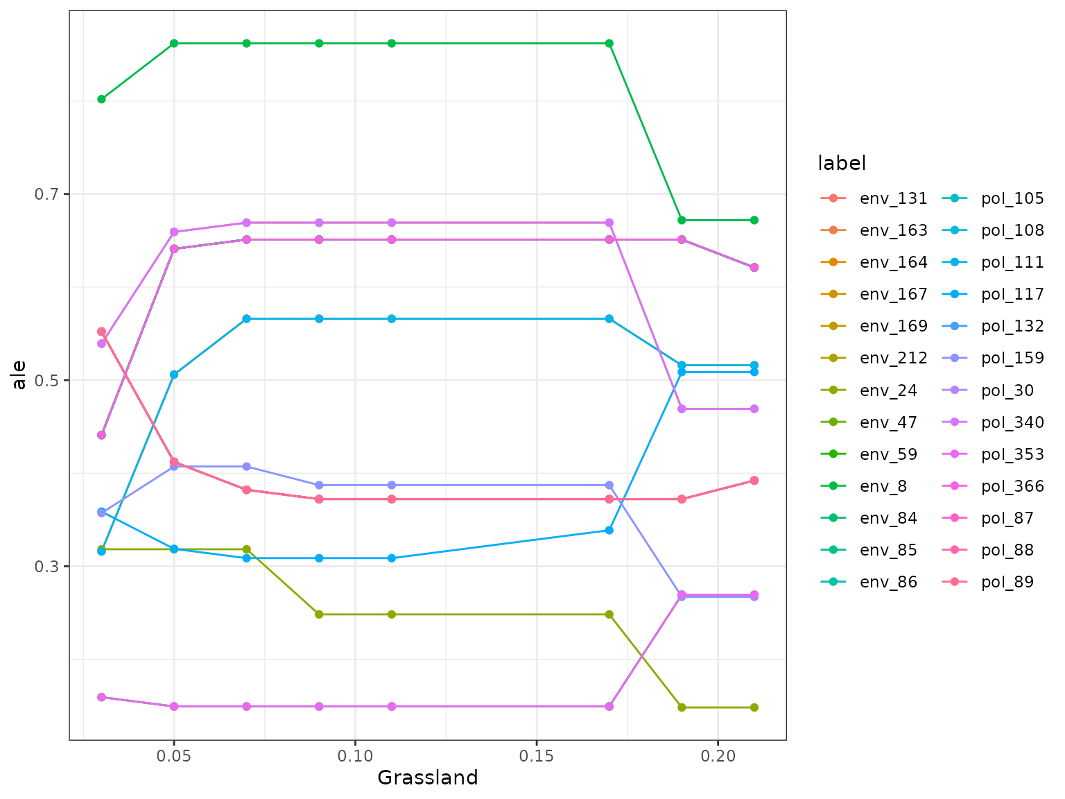
#> Press [enter] to continue to the global summary plot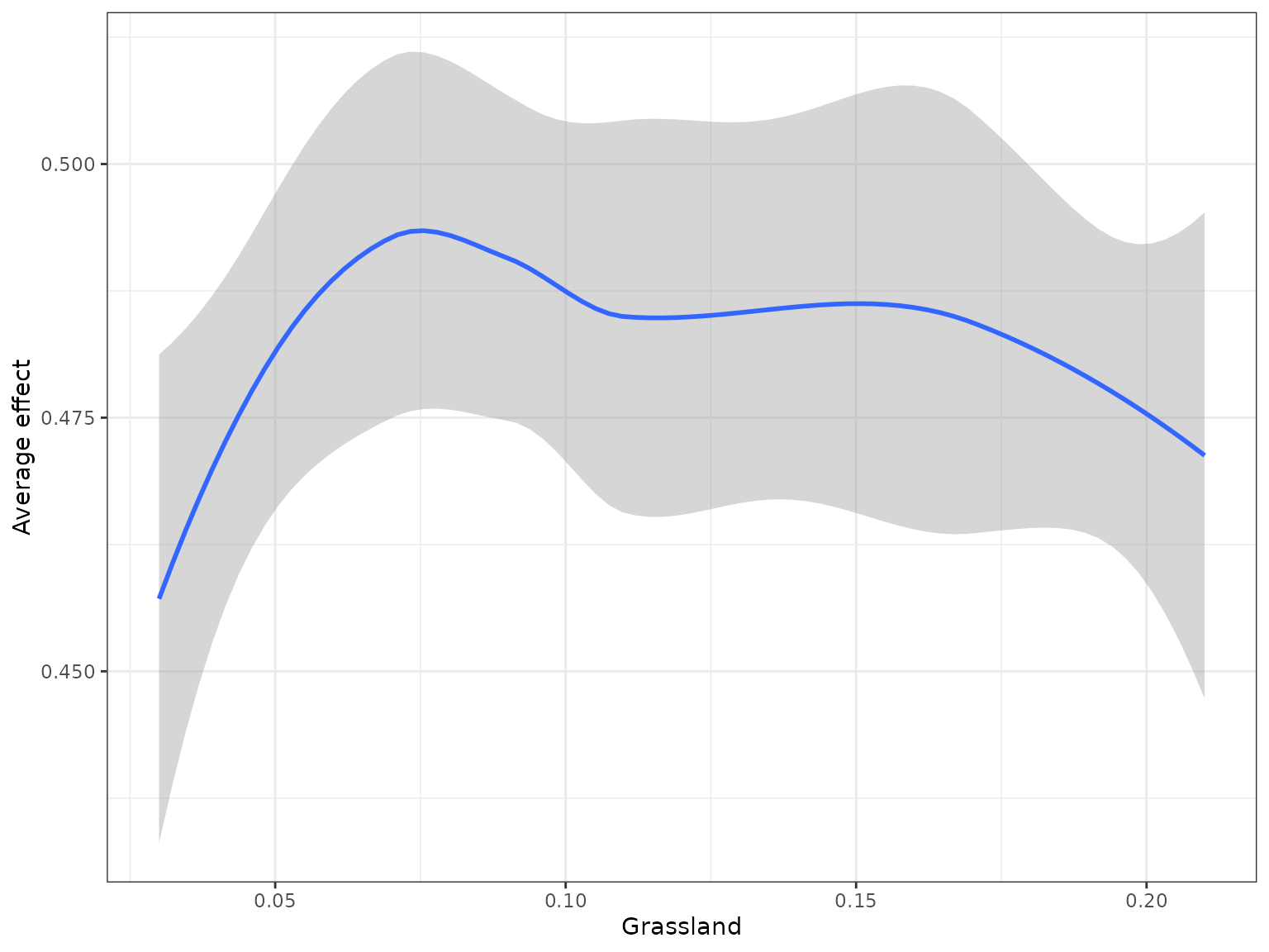
#the second plot is the cumulative turnover functionFinally, we can assess how features interact overall to shape genetic change.
interactions <-mrInteractions(yhats=yhats_rf,
                              X=X,
                              Y=Y,
                              num_bootstrap = 10,
                              feature = 'env_41',
                              top.int = 5)

interactions[[1]]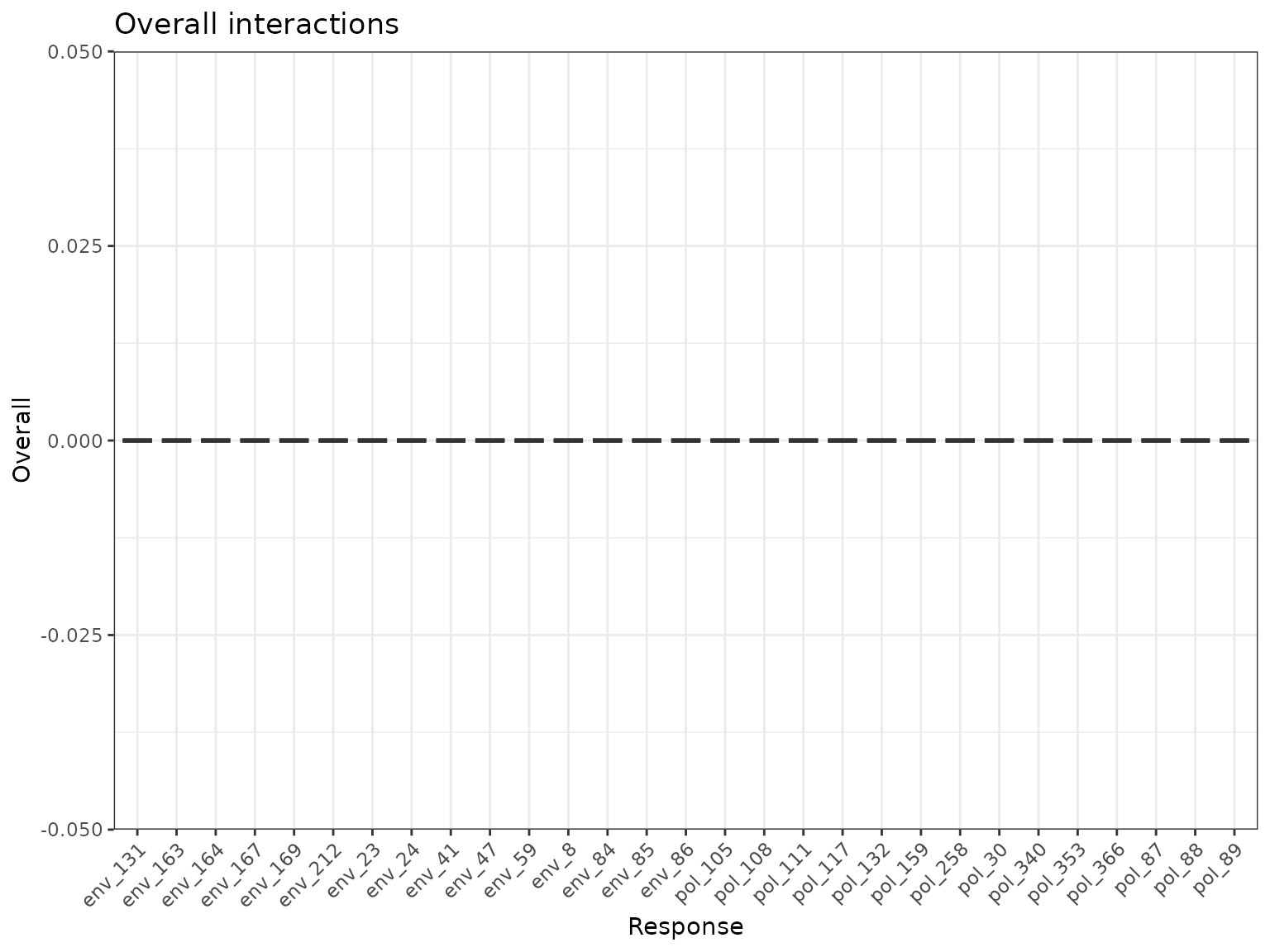
interactions[[2]] With this small data set with three predictors, interaction importance
isn’t particularly strong (H values > 0.1 on the y axis would
indicate that interactions are somewhat important). If you rerun this
with the complete set of predictors X there are many more. Also note,
that 10 bootstraps is not generally enough - particularly for small
datsets where stochasticity plays more of a role - at least 100 is
recommended.
With this small data set with three predictors, interaction importance
isn’t particularly strong (H values > 0.1 on the y axis would
indicate that interactions are somewhat important). If you rerun this
with the complete set of predictors X there are many more. Also note,
that 10 bootstraps is not generally enough - particularly for small
datsets where stochasticity plays more of a role - at least 100 is
recommended.
This is just an example of the tools can be applied to better interpret multi-response models and in turn gain insights into how landscape impacts genetic change. We’ve demonstrated that this package is modular and flexible, allowing future work on ‘tidymodels’ and interpretable machine learning to easily be incorporated. The predictions from these models, for example, can be used to identify individual SNPs that may be adaptive assess gene flow across space (future updates) or to help better formulate probabilistic models such as generalized dissimilarity models (GDMs).